This example solves for thermal convection within a full spherical shell domain.

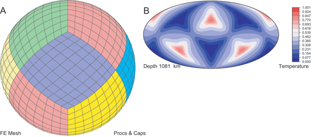
This example solves for thermal convection within a full spherical shell domain. The full spherical version of CitcomS.py is designed to run on a cluster that decomposes the spherical shell into 12 equal “caps” and then distributes the calculation for caps onto separate processors. To run CitcomS.py with the full solver parameter set, it is recommended that you have a minimum of 12 processors available on your cluster.

You will use cookbook1.cfg. The first set of parameters specifies that you are going to use the full spherical version of the solver. The default is to use the regional spherical version, so this must be set:

    solver = full

The second set of parameters specifies the number of time steps (101), how often full outputs of the computation are created (25), and the prefix of output filenames (cookbook1):

    steps = 101
    monitoringFrequency = 25
    datafile = cookbook1

The solver.ic facility controls the temperature field for the initial conditions. The last set of parameters includes the number of perturbations to the initial temperature (1), the number of nodal lines of the perturbation in the longitudinal direction, e.g., the spherical harmonic order (3), the number of nodal lines in the latitudinal direction, e.g., the spherical harmonic degree (2), which layer the pertubation is on (5), and the amplitude of the perturbation (0.05). Note that although the number of perturbations is assigned here as num_perturbations=1, that is actually the default value:

    num_perturbations = 1
    perturbl = 3
    perturbm = 2
    perturblayer = 5
    perturbmag = 0.05

This example is executed by typing '$ citcoms cookbook1.cfg'

Example: Global Model, cookbook1.cfg:

    [CitcomS]
    solver = full
    steps = 101                 ; number of time steps
    
    [CitcomS.controller]
    monitoringFrequency = 25    ; how often outputs are created
    
    [CitcomS.solver]
    datafile = cookbook1        ; prefix of output filenames
    
    [CitcomS.solver.ic]
    num_perturbations = 1
    perturbl = 3
    perturbm = 2
    perturblayer = 5
    perturbmag = 0.05 

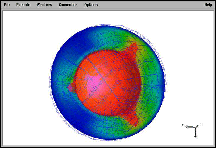
Once you have run the model, you can visualize the results using OpenDX, described in the previous chapter. When you invoke “Edit Visual Program,” select visFull.net.

You have generated a simple example of the full CitcomS.py model, with minimal parameter alterations. With a default Rayleigh number of 10⁵ and perturbation on the initial temperature field which has a degree-3 and an order-2 pattern, after 100 time steps, the convection pattern remains relatively steady.

As a side note, it is not required that 12 processors, with one spherical cap per processor, be used. As an end-member possibility, for example, 12 different jobs could be run on a single computer (n001 in this example) by invoking:

      $ citcoms cookbook1.cfg --launcher.nodegen="n%03d"\
      --launcher.nodelist=[1,1,1,1,1,1,1,1,1,1,1,1]

This is not particularly efficient, but it does illustrate the flexibility of both mpi and Pyre.