MAG

This content has been moved to hubzero. LJ Hwang 2020.12.28

MAG Software Page

The movie above shows the radial component of the geomagnetic field on the Earth's core-mantle boundary during a reverse-to-normal magnetic polarity transition, calculated using the MAG program. Red contours indicate outward magnetic flux, blue and black contours indicate inward magnetic flux. This animation represents approximately 10,000 years of simulated time. (original file)

A high-resolution version of the above phenomenon. (original hi-res, original low-res)

The following tutorials demonstrate (1) how to run the prepackaged benchmark data, and (2) how to produce a magnetic field reversal.

• Install MAG - The following tutorials assume you have already installed MAG following the instructions in Chapter 2 in the MAG User Manual.

• Delete, Move, or Rename Output Files - After each run, you must delete, move, or rename all of the output files in the current directory before re-running with the same “output” filename. Retaining same-named output files in the current directory causes MAG to crash.

• Changing Parameters - Physical and time-step parameters can be changed in the par-file namelist without re-compiling MAG. See Appendix B in the MAG User Manual for a list of the input parameter names and definitions. Grid parameters must be changed in param.f and MAG must be then re-compiled. There are some numerical restrictions on the grid parameter combinations, which are given in Appendix A.

Uncompress all files, and create a path (see Chapter 2 of MAG User Manual) Link the grid parameter file to param.f, which enters into most subroutines through “include” statements. For example, a grid parameter file named 'param32f4.f' (32 is the spherical harmonics truncation degree; 4 is the longitude symmetry) is linked using:

  $ ln -sf param32s4.f param.f 

Compile the program as follows (renaming the executable in line 2 is optional):

  $ make
  $ mv magx magx32s4  

MAG uses a standard input file. Background execute using par.XXX as the input file and .YYY as the output file's extension, e.g., '$ magx32s4 <par.XXX >p.YYY &', so to run with the benchmark input files (par.bnch0 or par.bnch1), the execution statement should be:

$ magx32s4 <par.bnch0 >p.bench0 &

If there is a problem with the input file list, it is often the final three lines; with some systems, a “$” may be required at the end.

MAG produces a series of output files. For example, when using input file par.bnch0 (the example in step 4) MAG generates: 'l.bench0, ls.bench0, g[i].bench0 and d[i].bench0', where i=0,1,2…9. See Appendix B in the MAG User Manual for details on MAG's output files. Compare your output files with the data provided in the directory ~/bench-data/data_bench0.

In this example, we produce a magnetic field reversal using MAG. The input parameter in the source directory for this case is ~/src/par.Rev. There is no longitudinal symmetry in this case, so when you compile MAG, use param32s1.f linking to param.f. The Ekman number is E=0.02, the Prandtl number is Pr=1 and the magnetic Prandtl number is Pm=10. The Rayleigh number is Ra=12000.

Link param32s1.f to param.f:

  $ ln -sf param32s1.f  param.f 

Compile the program with:

  $ make
  $ mv magx magx32s4 

Background execute using par.Rev as the input file and p.rev as the output file (Note: The output file's extension is specified in the par-file, e.g., here par.Rev specifies that the outfile should be named *filename*.rev):

  $ magx32s4 <par.Rev >p.rev &

MAG will then execute and produce datafiles in the same directory. See Appendix B in the MAG User Manual for details on MAG's output files.

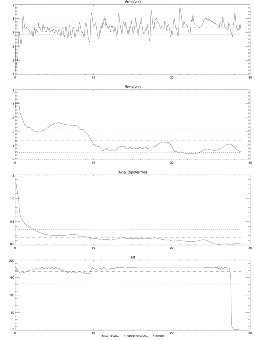
This case has run on 32-bit and 64-bit Intel processors. Figure 1 below shows a plot of mean velocity Vrms, mean magnetic field Brms, the axial dipole and the dipole tilt on the outer boundary. It indicated a magnetic field reversal between time steps 25 and 30.

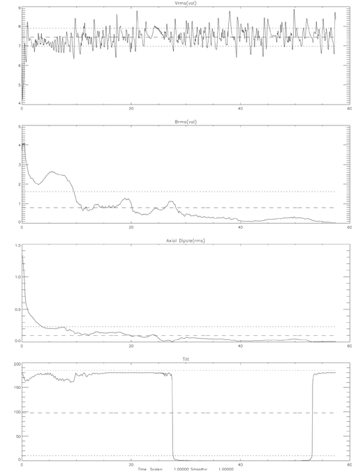
Figure 2 shows a longer run of MAG, where we see the magnetic field reversed again. At this time, the magnetic field had weakened substantially.

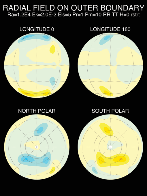
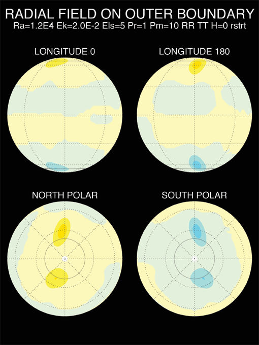
In Figures 3 and 4 (below), the top figure is the pole plot before the second field reversal and the bottom is the pole plot after the second field reversal.

An additional tutorial on creating a Reversal Dynamo movie is found in Chapter 5 of the MAG User Manual.