Sidebar
Table of Contents
SPECFEM3D
Development
If you want to contribute to the source code, please refer to https://github.com/geodynamics/specfem3d/wiki for details.
Tutorials
Step-by-step tutorials how to run SPECFEM3D simulations
Tutorial 1: Homogeneous halfspace
The following instructions assume that you have installed SPECFEM3D and familiarized yourself with how you will run the package based on your computer configuration, as detailed in the SPECFEM3D User manual (Chapter 2 provides installation help). Additionally, we will make use of an external, hexahedral mesher CUBIT. Please make sure you have these packages installed on your system.
The example is distributed with the package under the examples/ directory. However, you might need to edit these example scripts slightly to launch them on your system.
Homogeneous halfspace
This is a step-by-step tutorial how to create a mesh for a homogeneous halfspace, export it into a SPECFEM3D file format and run the mesh partitioning and database generation.
Meshing
In the following, we will run a python script within CUBIT to create the needed mesh files for the partitioner.
1. change your working directory to the example folder:
[]$ cd SPECFEM3D/examples/homogeneous_halfspace
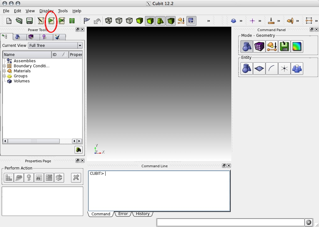
2. start the graphical user interface (GUI) of CUBIT:
[homogeneous_halfspace]$ claro
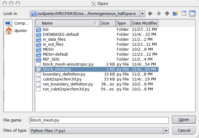
3. run the python file “block_mesh.py”:
use the (Play Journal File) button and open the file 'block_mesh.py'
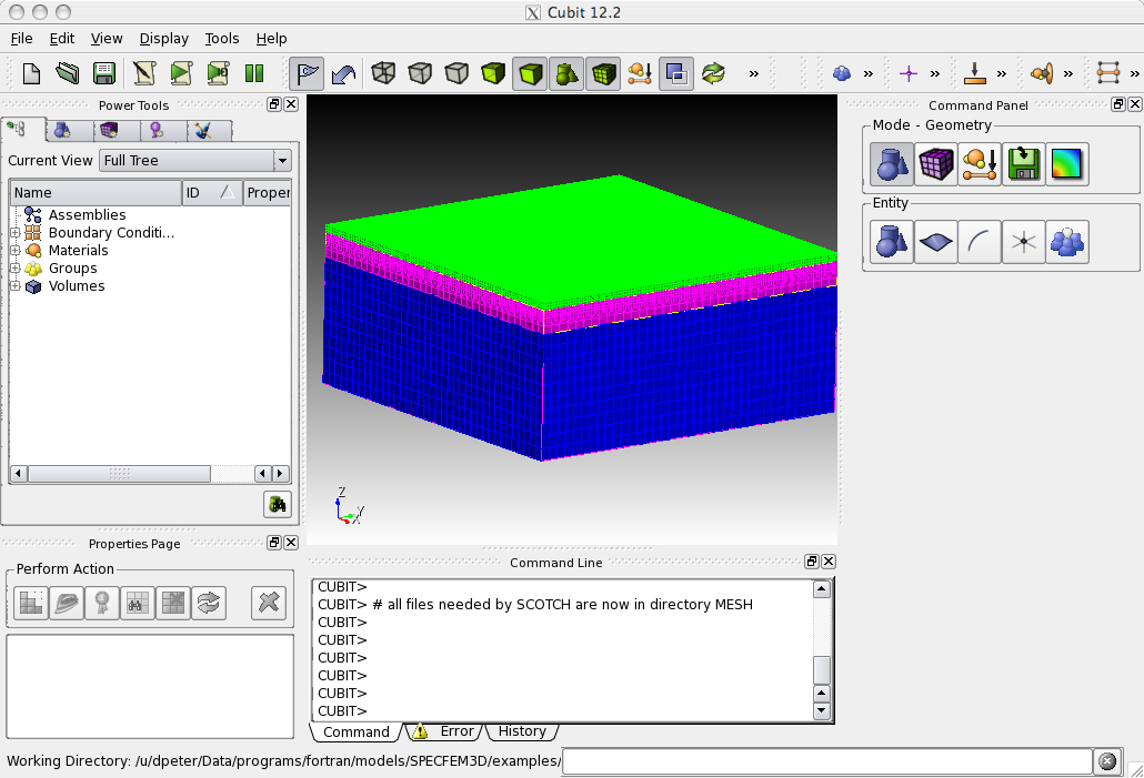
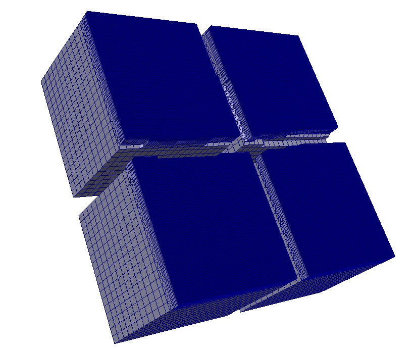
4. in case the script executed successfully, it should create you a single volume with a regular mesh
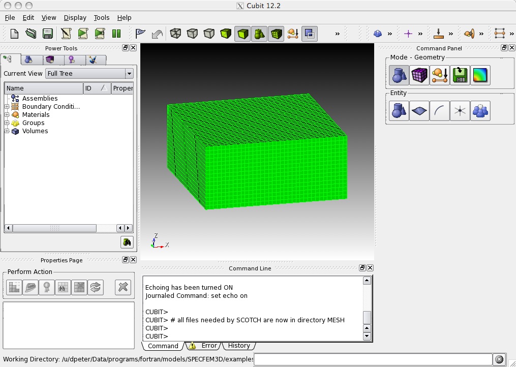
check that the script created a new folder “MESH/” containing the files:
[homogeneous_halfspace]$ ls -1 MESH/
absorbing_surface_file_bottom
absorbing_surface_file_xmax
absorbing_surface_file_xmin
absorbing_surface_file_ymax
absorbing_surface_file_ymin
free_surface_file
materials_file
mesh_file
nodes_coords_file
nummaterial_velocity_file
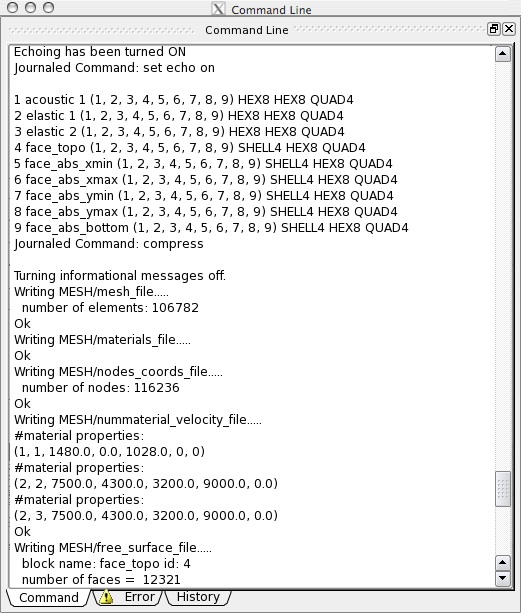
you can also check if the export was successful by examining the output in the Command line window of CUBIT. The sensitive part should look like

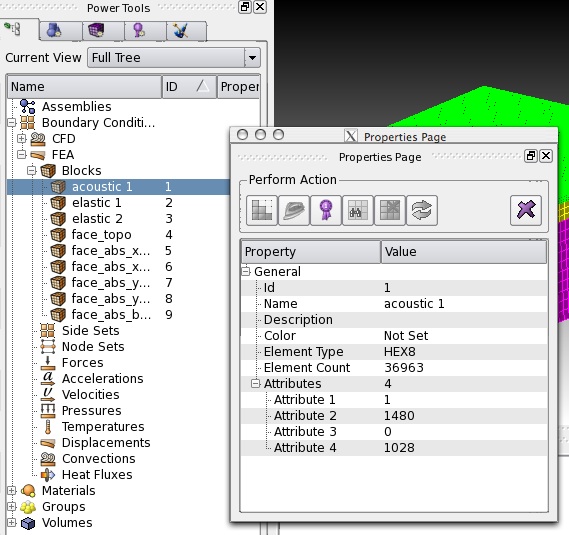
5. optionally, you could modify the material properties of the halfspace, by going to change the block properties
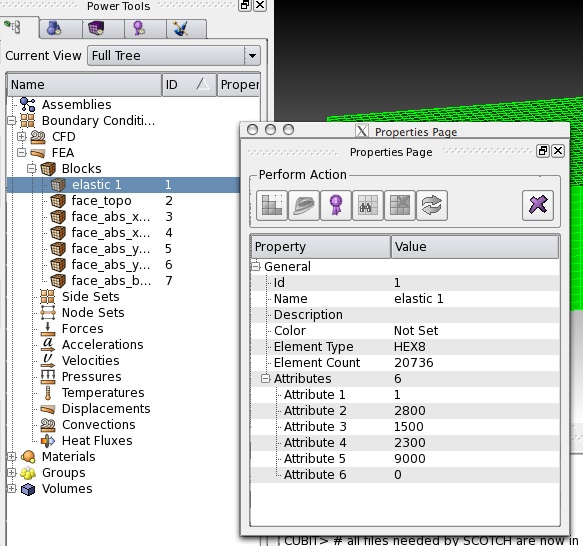
the following table applies for elastic material properties:
| Name | block name must start with “elastic” for elastic materials followed by a unique identifier material_id |
|---|---|
| Attribute 1 | Material ID |
| Attribute 2 | P-wave speed |
| Attribute 3 | S-wave speed |
| Attribute 4 | Density |
| Attribute 5 | Quality factor |
| Attribute 6 | Anisotropy flag |
Once you changed the properties, you will have to re-export the mesh. This can be done, using the script run_cubit2specfem3d.py:
use the (Play Journal File) button and open the file "run_cubit2specfem3d.py"
This should refresh the files in directory “MESH/”.
Setting up example folder for simulations
We will set up the example folder for simulation runs:
* databases directory:
create a directory in_out_files/DATABASES_MPI/ into which you will put the mesh partitions:
[]$ cd SPECFEM3D/examples/homogeneous_halfspace
[homogeneous_halfspace]$ mkdir -p in_out_files/DATABASES_MPI
* parameter files:
make sure you have the parameter files in a local directory in_data_files/ for the example:
[homogeneous_halfspace]$ ls -1 in_data_files/
Par_file
CMTSOLUTION
STATIONS
these files should already be provided in the example folder.
* executables: compile the executables in the root directory:
[]$ cd SPECFEM3D/
[SPECFEM3D]$ make
in case the compilation was successful, it will create the executables xdecompose_mesh_SCOTCH, xgenerate_databases and xspecfem3D in the bin/ directory
and create a local directory bin/ to link the executables from the root directory:
[]$ cd SPECFEM3D/examples/homogeneous_halfspace
[homogeneous_halfspace]$ mkdir -p bin
[homogeneous_halfspace]$ cd bin/
[bin]$ ln -s ../../../bin/xdecompose_mesh_SCOTCH
[bin]$ ln -s ../../../bin/xgenerate_databases
[bin]$ ln -s ../../../bin/xspecfem3D
All these steps and the following decomposition, database generation and solver run are put in a process.sh bash script file in the example folder. You can simply run the script:
[homogeneous_halfspace]$ ./process.sh
to do the setup and following steps for you. Please modify and adapt the script to your needs.
Mesh partitioning
In this example, we will partition the mesh for 4 CPU cores.
run the mesh partitioner:
[homogeneous_halfspace]$ ./bin/xdecompose_mesh_SCOTCH 4 MESH/ in_out_files/DATABASES_MPI/
check that this created the mesh partitions:
[homogeneous_halfspace]$ ls -1 in_out_files/DATABASES_MPI/
proc000000_Database
proc000001_Database
proc000002_Database
proc000003_Database

You are done.
Database generation
Next, you will need to create the mesh databases.
1. in case you can run parallel programs on your desktop (needs an MPI installation), you can run the executable like:
[homogeneous_halfspace]$ cd bin/
[bin]$ mpirun -np 4 ./xgenerate_databases
otherwise, you will need to modify and adapt one of the cluster scripts provided in the SPECFEM3D/utils/Cluster/ directory.
2. check the output file in_out_files/OUTPUT_FILES/output_mesher.txt to see if the databases were generated successfully.
The output file contains the suggested time step for your mesh:
Verification of simulation parameters
...
Minimum period resolved =    2.115564
**Maximum suggested time step =   6.8863556E-02**
Forward simulation
To run a forward simulation, do the following:
1. make sure, you have the parameter files in the directory in_data_files/.
Most parameters in the Par_file should be set before running the database generation.
The following may be changed after running xgenerate_databases:
# forward or adjoint simulation
SIMULATION_TYPE                 = 1   # 1 = forward, 2 = adjoint, 3 = both simultaneously
NOISE_TOMOGRAPHY                = 0   # 0 = earthquake simulation,  1/2/3 = three steps in noise simulation
SAVE_FORWARD                    = .false.

# time step parameters
NSTEP                           = 1000
DT                              = 0.05

# absorbing boundary conditions for a regional simulation
ABSORBING_CONDITIONS            = .false.

# save AVS or OpenDX movies
MOVIE_SURFACE                   = .false.
MOVIE_VOLUME                    = .false.
NTSTEP_BETWEEN_FRAMES           = 200
CREATE_SHAKEMAP                 = .false.
SAVE_DISPLACEMENT               = .false.
USE_HIGHRES_FOR_MOVIES          = .false.
HDUR_MOVIE                      = 0.0

# interval at which we output time step info and max of norm of displacement
NTSTEP_BETWEEN_OUTPUT_INFO      = 500

# interval in time steps for writing of seismograms
NTSTEP_BETWEEN_OUTPUT_SEISMOS   = 10000

# interval in time steps for reading adjoint traces
NTSTEP_BETWEEN_READ_ADJSRC      = 0      # 0 = read the whole adjoint sources at the same time

# print source time function
PRINT_SOURCE_TIME_FUNCTION      = .false.
2. in case you can run parallel programs on your desktop (needs an MPI installation), you can run the executable like:
[homogeneous_halfspace]$ cd bin/
[bin]$ mpirun -np 4 ./xspecfem3D
this example should take about 5 minutes to finish the simulation.
3. check the output file output_solver.txt in the output directory in_out_files/OUTPUT_FILES/ to see if the forward simulation was successfully finishing.
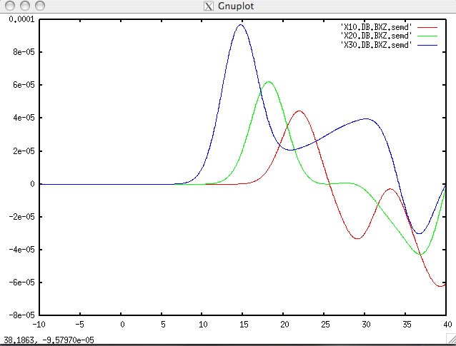
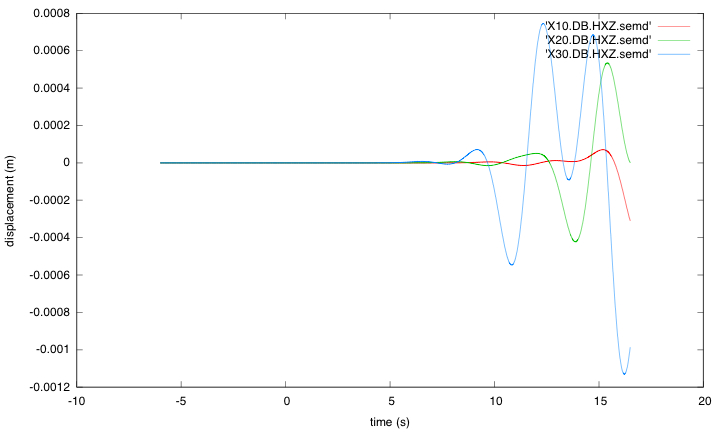
the seismograms will look like this, using gnu plot:
gnuplot> plot "X10.DB.BXZ.semd" w l,"X20.DB.BXZ.semd" w l,"X30.DB.BXZ.semd" w l
Tutorial 2: Waterlayered halfspace
The following instructions assume that you have installed SPECFEM3D and familiarized yourself with how you will run the package based on your computer configuration, as detailed in the SPECFEM3D User manual (Chapter 2 provides installation help). Additionally, we will make use of an external, hexahedral mesher CUBIT. Please make sure you have these packages installed on your system.
The example is distributed with the package under the examples/ directory. However, you might need to edit these example scripts slightly to launch them on your system.
Waterlayered halfspace
This is a step-by-step tutorial how to create a mesh for a layered halfspace with a water layer on top, export it into a SPECFEM3D file format and run the mesh partitioning and database generation.
Meshing
In the following, we will run a python script within CUBIT to create the needed mesh files for the partitioner.
1. change your working directory to the example folder:
[]$ cd SPECFEM3D/examples/waterlayered_halfspace
2. start the graphical user interface (GUI) of CUBIT:
[waterlayered_halfspace]$ claro
3. run the python file:
use the (Play Journal File) button and open the file "waterlayer_mesh_boundary_fig8.py"
4. in case the script executed successfully, it should create you three volumes with a refined mesh for the top layer, a triplication layer and a coarser mesh layer at the bottom:
check that the script created a new folder “MESH/” containing the files:
[waterlayered_halfspace]$ ls -1 MESH/
absorbing_surface_file_bottom
absorbing_surface_file_xmax
absorbing_surface_file_xmin
absorbing_surface_file_ymax
absorbing_surface_file_ymin
free_surface_file
materials_file
mesh_file
nodes_coords_file
nummaterial_velocity_file
you can also check if the export was successful by examining the output in the Command line window of CUBIT. The sensitive part should look like
5. optionally, you could modify the material properties of the model, either in CUBIT or in the newly created material file:
* changing the block properties in CUBIT
the following table applies for acoustic material properties:
| Name | block name must start with “acoustic” for acoustic materials followed by a unique identifier material_id |
|---|---|
| Attribute 1 | Material ID |
| Attribute 2 | P-wave speed |
| Attribute 3 | S-wave speed is ignored, set to zero |
| Attribute 4 | Density |
the following table applies for elastic material properties:
| Name | block name must start with “elastic” for elastic materials followed by a unique identifier material_id |
|---|---|
| Attribute 1 | Material ID |
| Attribute 2 | P-wave speed |
| Attribute 3 | S-wave speed |
| Attribute 4 | Density |
| Attribute 5 | Quality factor |
| Attribute 6 | Anisotropy flag |
Once you changed the properties, you will have to re-export the mesh. This can be done, using the script run_cubit2specfem3d.py:
use the (Play Journal File) button and open the file "run_cubit2specfem3d.py"
This should refresh the files in directory “MESH/”.
* directly modifing the file nummaterial_velocity_file in the MESH/ directory:
1   1          1028.000000          1480.000000             0.000000             0.000000  0
2   2          3200.000000          7500.000000          4300.000000          9000.000000  0
2   3          3200.000000          7500.000000          4300.000000          9000.000000  0
this file defines the material properties. the format is:
| Domain_id | Material_id | Density | P-wave speed | S-wave speed | Quality factor | Anisotropy_flag |
|---|---|---|---|---|---|---|
| 1 = acoustic, | unique material | density | wave speed in m/s | wave speed in m/s | Quality factor, | flag for anisotropy model, |
| 2 = elastic | identifier | in kg/m3 | (ignored for acoustic materials) | 0 = no attenuation | 0 = no anisotropy |
Setting up example folder for simulations
We will set up the example folder for simulation runs:
* databases directory:
create a directory in_out_files/DATABASES_MPI/ into which you will put the mesh partitions:
[]$ cd SPECFEM3D/examples/waterlayered_halfspace
[waterlayered_halfspace]$ mkdir -p in_out_files/DATABASES_MPI
* parameter files:
make sure you have the parameter files in a local directory in_data_files/ for the example:
[waterlayered_halfspace]$ ls -1 in_data_files/
Par_file
CMTSOLUTION
STATIONS
these files should already be provided in the example folder.
* executables: compile the executables in the root directory:
[]$ cd SPECFEM3D/
[SPECFEM3D]$ make
in case the compilation was successful, it will create the executables xdecompose_mesh_SCOTCH, xgenerate_databases and xspecfem3D in the bin/ directory
and create a local directory bin/ to link the executables from the root directory:
[]$ cd SPECFEM3D/examples/waterlayered_halfspace
[waterlayered_halfspace]$ mkdir -p bin
[waterlayered_halfspace]$ cd bin/
[bin]$ ln -s ../../../bin/xdecompose_mesh_SCOTCH
[bin]$ ln -s ../../../bin/xgenerate_databases
[bin]$ ln -s ../../../bin/xspecfem3D
All these steps and the following decomposition, database generation and solver run are put in a process.sh bash script file in the example folder. You can simply run the script:
[waterlayered_halfspace]$ ./process.sh
to do the setup and following steps for you. Please modify and adapt the script to your needs.
Mesh partitioning
In this example, we will partition the mesh for 4 CPU cores.
run the mesh partitioner:
[waterlayered_halfspace]$ ./bin/xdecompose_mesh_SCOTCH 4 MESH/ in_out_files/DATABASES_MPI/
check that this created the mesh partitions:
[waterlayered_halfspace]$ ls -1 in_out_files/DATABASES_MPI/
proc000000_Database
proc000001_Database
proc000002_Database
proc000003_Database
You are done.
Database generation
Next, you will need to create the mesh databases.
1. in case you can run parallel programs on your desktop (needs an MPI installation), you can run the executable like:
[waterlayered_halfspace]$ cd bin/
[bin]$ mpirun -np 4 ./xgenerate_databases
otherwise, you will need to modify and adapt one of the cluster scripts provided in the SPECFEM3D/utils/Cluster/ directory.
2. check the output file in_out_files/OUTPUT_FILES/output_mesher.txt to see if the databases were generated successfully.
The output file contains the suggested time step for your mesh:
Verification of simulation parameters
...
Minimum period resolved =   1.632425
**Maximum suggested time step =   5.1801954E-03**
Forward simulation
To run a forward simulation, do the following:
1. make sure, you have the parameter files in the directory in_data_files/.
Most parameters in the Par_file should be set before running the database generation.
The following may be changed after running xgenerate_databases:
# forward or adjoint simulation
SIMULATION_TYPE                 = 1   # 1 = forward, 2 = adjoint, 3 = both simultaneously
NOISE_TOMOGRAPHY                = 0   # 0 = earthquake simulation,  1/2/3 = three steps in noise simulation
SAVE_FORWARD                    = .false.

# time step parameters
NSTEP                           = 4500
DT                              = 0.005

# absorbing boundary conditions for a regional simulation
ABSORBING_CONDITIONS            = .true.

# save AVS or OpenDX movies
MOVIE_SURFACE                   = .false.
MOVIE_VOLUME                    = .false.
NTSTEP_BETWEEN_FRAMES           = 200
CREATE_SHAKEMAP                 = .false.
SAVE_DISPLACEMENT               = .false.
USE_HIGHRES_FOR_MOVIES          = .false.
HDUR_MOVIE                      = 0.0

# interval at which we output time step info and max of norm of displacement
NTSTEP_BETWEEN_OUTPUT_INFO      = 500

# interval in time steps for writing of seismograms
NTSTEP_BETWEEN_OUTPUT_SEISMOS   = 10000

# interval in time steps for reading adjoint traces
NTSTEP_BETWEEN_READ_ADJSRC      = 0      # 0 = read the whole adjoint sources at the same time

# print source time function
PRINT_SOURCE_TIME_FUNCTION      = .false.
2. in case you can run parallel programs on your desktop (needs an MPI installation), you can run the executable like:
[waterlayered_halfspace]$ cd bin/
[bin]$ mpirun -np 4 ./xspecfem3D
note, this example should take about 1 hour 45 minutes to finish the simulation.
3. check the output file output_solver.txt in the output directory in_out_files/OUTPUT_FILES/
to see if the forward simulation was successfully finishing.
the seismograms will look like this, using gnuplot:
gnuplot> plot "X10.DB.BXZ.semd" w l,"X20.DB.BXZ.semd" w l,"X30.DB.BXZ.semd" w l
Tutorial 3: Mount St. Helens
The following instructions assume that you have installed SPECFEM3D and familiarized yourself with how you will run the package based on your computer configuration, as detailed in the “SPECFEM3D User manual”:http://www.geodynamics.org/wsvn/cig/seismo/3D/SPECFEM3D/trunk/doc/USER_MANUAL/manual_SPECFEM3D.pdf?op=file&rev=0&sc=0 (Chapter 2 provides installation help). Additionally, we will make use of an external, hexahedral mesher CUBIT. Please make sure you have these packages installed on your system.
The example is distributed with the package under the examples/ directory. However, you might need to edit these example scripts slightly to launch them on your system.
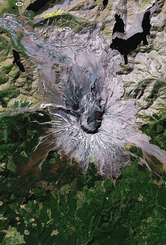
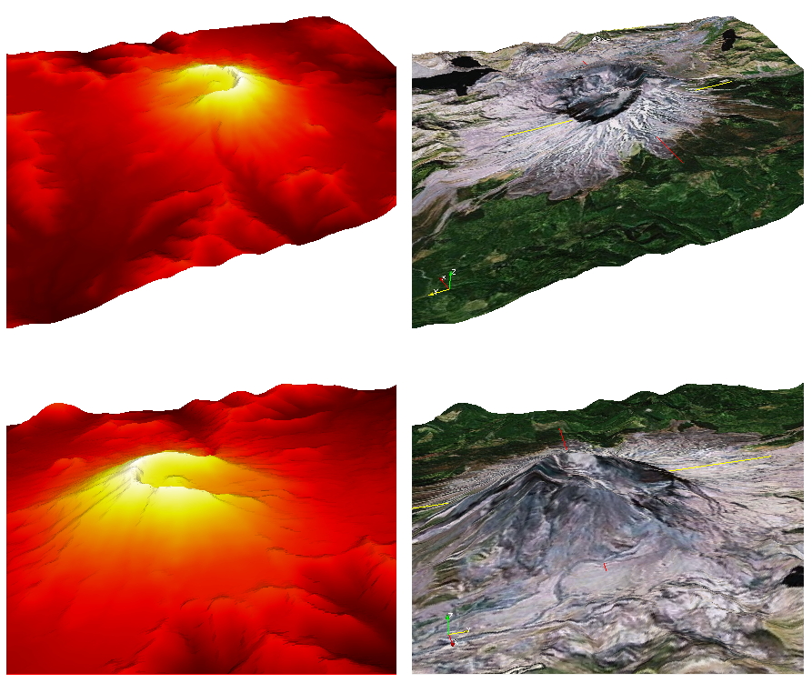
Mount St. Helens
This is a step-by-step tutorial how to create a mesh for a region around Mount St. Helens, export it into a SPECFEM3D file format and run the mesh partitioning and database generation.
Change to the example directory
[]$ cd SPECFEM3D/examples/Mount_StHelens
Please also see the README file in this example directory. An example topography file “ptopo.mean.utm” is provided as well, in the following we explain in detail how to construct such a file.
Downloading topography data
You can get SRTM 90m Digital Elevation Data for a region of interest at: http://srtm.csi.cgiar.org
For this example, we choose Mount St.Helens as region of interest.
Mount St. Helens is located at: 46.197 N 122.186 W
This region is contained in a downloadable file srtm_12_03.zip, which you will have to download from
http://srtm.csi.cgiar.org/SELECTION/inputCoord.asp
using the region of interest:
Latitude min: 45 N  max: 50 N
Longitude min: 125 W max: 120 W
unzipping the file
[Mount_StHelens]$ unzip srtm_12_03.zip
leads to:
..
srtm_12_03.tif
..
Converting Geotif topography data
To convert the Geotif-file into an longitude/latitude/elevation format, you can use the package FWTools at: http://fwtools.maptools.org/
Install the package and use their gdal2xyz executable to extract the tif file into xyz format:
[Mount_StHelens]$ FWTools-2.0.6/bin_safe/gdal2xyz.py srtm_12_03.tif > srtm_12_03.xyz
the newly created file srtm_12_03.xyz has now the format:
#longitude #latitude #elevation (m)
the file size is ~ 963 MB.
Extracting the region of interest
To further extract and manipulate the topography data, you can use the package GMT at: http://gmt.soest.hawaii.edu/
For our purpose, the region of interest will be:
\ -R-122.3/-122.1/46.1/46.3//
that is a region of ~23 km x 23 km extent.
Using the blockmean executable from the GMT package, we extract and interpolate the topography data for the detailed region, using an interpolated grid spacing of 0.006 degrees (~ 700 m):
[Mount_StHelens]$ blockmean srtm_12_03.xyz -R-122.3/-122.1/46.1/46.3 -I0.006/0.006 > ptopo.mean.xyz
This will create a new file ptopo.mean.xyz with a longitude/latitude/elevation format of the region of interest
Converting to Cartesian coordinates
Since the CUBIT mesh will need Cartesian coordinates, we convert the topography file from longitude/latitude/elevation to X/Y/Z coordinates using a UTM projection.
Mount St.Helens lies in the UTM zone: 10 (T).
Use the script “convert_lonlat2utm.pl” provided in this example folder:
[Mount_StHelens]$ ./convert_lonlat2utm.pl ptopo.mean.xyz 10 > ptopo.mean.utm
to create a new file ptopo.mean.utm which will have a file format:
#UTM_X (m) #UTM_Y (m) #Z (m)
Meshing
In the following, we will run a python script within CUBIT to create the needed mesh files for the partitioner.
1. if not done so yet, change your working directory to the example folder:
[]$ cd SPECFEM3D/examples/Mount_StHelens
2. start the graphical user interface (GUI) of CUBIT:
[Mount_StHelens]$ claro
3. run the python file “read_topo.py”:
use the (Play Journal File) button and open the file 'read_topo.py'
The script creates a topography surface topo.stl in STL file format as well as topo.cub based on file ptopo.mean.utm.
4. run the python file “mesh_mount.py”:
use the (Play Journal File) button and open the file 'mesh_mount.py'
In case the script executed successfully, it should create you a single volume with a refined mesh for the top layer, a triplication layer and a coarser mesh at the bottom.
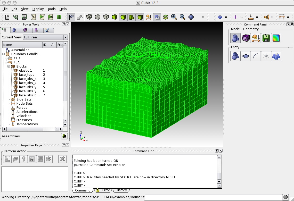
check that the script created a new folder “MESH/” containing the files:
[Mount_StHelens]$ ls -1 MESH/
absorbing_surface_file_bottom
absorbing_surface_file_xmax
absorbing_surface_file_xmin
absorbing_surface_file_ymax
absorbing_surface_file_ymin
free_surface_file
materials_file
mesh_file
nodes_coords_file
nummaterial_velocity_file
you can also check if the export was successful by examining the output in the Command line window of CUBIT.
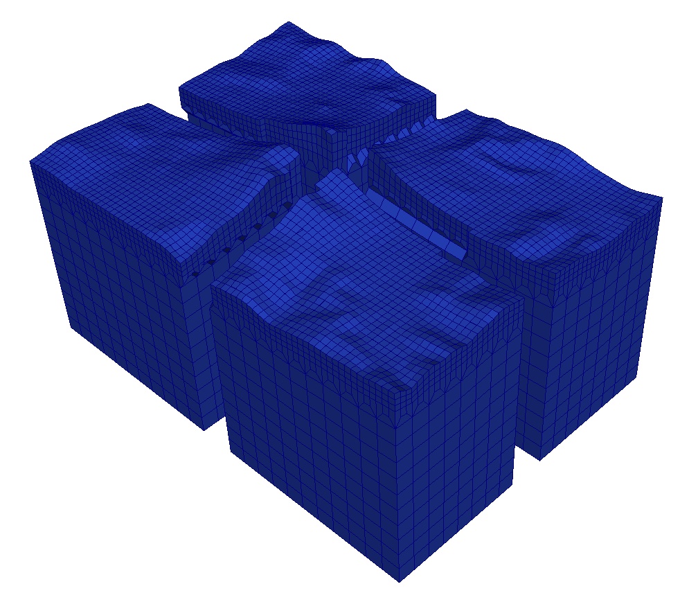
Setting up example folder for simulations
We will set up the example folder for simulation runs: All the steps and following decomposition, database generation and solver run are put in a process.sh bash script file in the example folder.
1. In case you can run parallel programs on your desktop (needs an MPI installation), you can simply run the script:
[Mount_StHelens]$ ./process.sh
to do the setup and following steps for you. The simulation will run on 4 CPU cores by default. Please modify and adapt the script to your needs.
Note, this example should take about 15 minutes to finish the simulation.
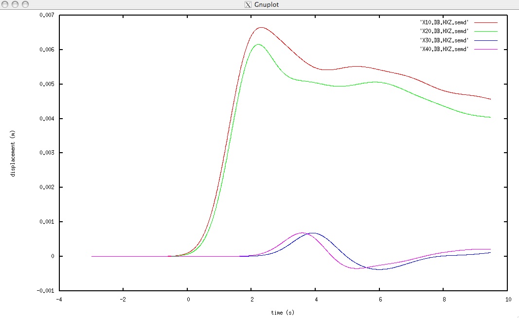
2. check the output file output_solver.txt in the output directory in_out_files/OUTPUT_FILES/ to see if the forward simulation was successfully finishing.
the seismograms will look like this, using gnuplot:
gnuplot> plot "X10.DB.HXZ.semd" w l,"X20.DB.HXZ.semd" w l,"X30.DB.HXZ.semd" w l,"X40.DB.HXZ.semd" w l