SPECFEM3D Globe Software Page

If you want to contribute to the source code, please refer to https://github.com/geodynamics/specfem3d/wiki for details.

This is a step-by-step tutorial how to create a mesh for a global simulation and run a forward simulation.

The following instructions assume that you have installed SPECFEM3D_GLOBE and familiarized yourself with how you will run the package based on your computer configuration, as detailed in the SPECFEM3D_GLOBE User manual (Chapter 2 provides installation help). Please make sure you have the package installed on your system.

The example is distributed with the package under the EXAMPLES/ directory. However, you might need to edit these example scripts slightly to launch them on your system.

This is a step-by-step tutorial how to create a mesh for a global simulation and run a single forward simulation.

We will set up the example folder for simulation runs:

* databases directory: create a directory DATABASES_MPI/ into which you will put the mesh partitions:

[]$ cd SPECFEM3D_GLOBE/EXAMPLES/global_s362ani/
[global_s362ani]$ mkdir -p DATABASES_MPI

Make sure this folder is accessible by the compute nodes on your system. The example will search for this folder in the current example directory. Depending on your system setup, you may also create this as a symbolic link to a local scratch directory /scratch/DATABASES_MPI.

* parameter files: make sure you have the parameter files in a local directory DATA/ for the example:

[global_s362ani]$ ls -1 DATA/
Par_file
CMTSOLUTION
STATIONS

these files should already be provided in the example folder.

* executables: compile the executables in the root directory:

[]$ cd SPECFEM3D_GLOBE/
[SPECFEM3D_GLOBE]$ make

this assumes that you run the configuration beforehand by ./configure (see the manual for further configuration options). In case the compilation was successful, it will create the main executables xmeshfem3D and xspecfem3D in the bin/ directory

create a local directory bin/ to link the executables from the root directory:

[]$ cd SPECFEM3D_GLOBE/EXAMPLES/global_s362ani
[global_s362ani]$ mkdir -p bin    
[global_s362ani]$ cd bin/
[bin]$ ln -s ../../bin/xmeshfem3D
[bin]$ ln -s ../../bin/xspecfem3D

All these steps and the following mesher and solver runs are put in a process.sh bash script file in the example folder. You can simply run the script:

[global_s362ani]$ ./process.sh

to do the setup and following steps for you. The script uses a PBS scheduler to submit the corresponding cluster job. Please modify and adapt the script to your needs.

You will need to create the mesh databases before you can run the solver.

1. the example will run the mesher in parallel on 150 CPUs. A script go_mesher_solver_pbs.bash is provided in this example folder to do this via a PBS job scheduler. You may adapt also one of the cluster scripts provided in the SPECFEM3D_GLOBE/UTILS/Cluster/ directory for this purpose.

Note: This example script will submit one single job script which contains both the meshing run and the forward solver run together. This is especially useful in case your DATABASES_MPI folder is only locally accessible on the cluster nodes (e.g. local scratch disk space) and allows you to run both meshing and forward simulation without the need to store all the created mesh database files in a globally accessible repository.

2. make sure, you have the parameter file Par_file in the local directory DATA/. This example will use the following parameter setup for the global simulation:

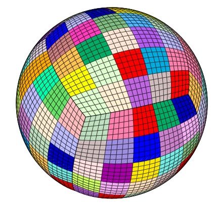
# forward or adjoint simulation
SIMULATION_TYPE                 = 1   # 1 = forward, 2 = adjoint, 3 = both simultaneously
NOISE_TOMOGRAPHY                = 0   # 0 = earthquake simulation,  1/2/3 = three steps in noise simulation
SAVE_FORWARD                    = .false.  

# number of chunks (1,2,3 or 6)
NCHUNKS                         = 6
...
# number of elements at the surface along the two sides of the first chunk
# (must be multiple of 16 and 8 * multiple of NPROC below)
NEX_XI                          = 240
NEX_ETA                         = 240

# number of MPI processors along the two sides of the first chunk
NPROC_XI                        = 5
NPROC_ETA                       = 5
...
# 3D model
MODEL                           = s362ani
...
# path to store the local database files on each node
LOCAL_PATH                      = ./DATABASES_MPI
...

The number of spectral elements per chunk in both XI and ETA directions is 240. To obtain the shortest period resolved in the seismograms, you would determine:

shortest period ~ (256 / NEX_XI ) * 17

thus for this example, they are accurate down to approximately 18 s periods.

Once the mesher completed, check the output file OUTPUT_FILES/output_mesher.txt to see if the databases were generated successfully. The output file contains various mesh information, including the time step size used for your forward simulation:

time-stepping of the solver will be:   0.161500000000000

To run a forward simulation, do the following:

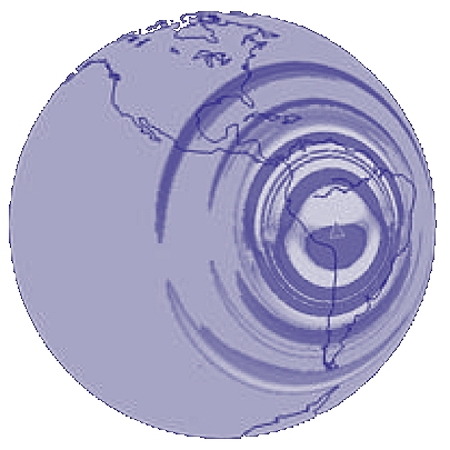
1. set an earthquake source by modifying the file CMTSOLUTION in the directory DATA/. this example will use a CMT solution for a deep earthquake (647.1 km depth) which took place in Bolivia in June, 1994.

You can obtain more CMT solutions from the Global Centroid-Moment Tensor project catalog.

2. place your stations by modifying the file STATIONS in the directory DATA/. this example will use a very small subset of seismic stations in international networks IRIS/IDA (II) and IRIS/USGS (IU) as well as station PAS located in Pasadena, CA, USA.

You can obtain more station information from the International Federation of Digital Seismograph Networks (FDSN).

Please see the SPECFEM3D_GLOBE User manual for more detailed informations of how to specify the source and stations.

3. make sure, you have the parameter files in the directory DATA/. Most parameters in the Par_file should be set before running the mesher xmeshfem3D. The following parameters are important for this example forward simulation:

# forward or adjoint simulation
SIMULATION_TYPE                 = 1   # 1 = forward, 2 = adjoint, 3 = both simultaneously
NOISE_TOMOGRAPHY                = 0   # 0 = earthquake simulation,  1/2/3 = three steps in noise simulation
SAVE_FORWARD                    = .false.  

# number of chunks (1,2,3 or 6)
NCHUNKS                         = 6
...
# number of MPI processors along the two sides of the first chunk
NPROC_XI                        = 5
NPROC_ETA                       = 5
...
# 3D model
MODEL                           = s362ani

# parameters describing the Earth model
OCEANS                          = .true.
ELLIPTICITY                     = .true.
TOPOGRAPHY                      = .true.
GRAVITY                         = .true.
ROTATION                        = .true.
ATTENUATION                     = .true.

# absorbing boundary conditions for a regional simulation
ABSORBING_CONDITIONS            = .false.

# record length in minutes
RECORD_LENGTH_IN_MINUTES        = 15.0d0
...
# path to store the local database files on each node
LOCAL_PATH                      = ./DATABASES_MPI
...  
# output format for the seismograms (one can use either or all of the three formats)
OUTPUT_SEISMOS_ASCII_TEXT       = .true.  
...

this example will use a single job script go_mesher_solver_pbs.bash to run mesher and solver together. The solver should take about 1 hour 45 minutes to finish the simulation.

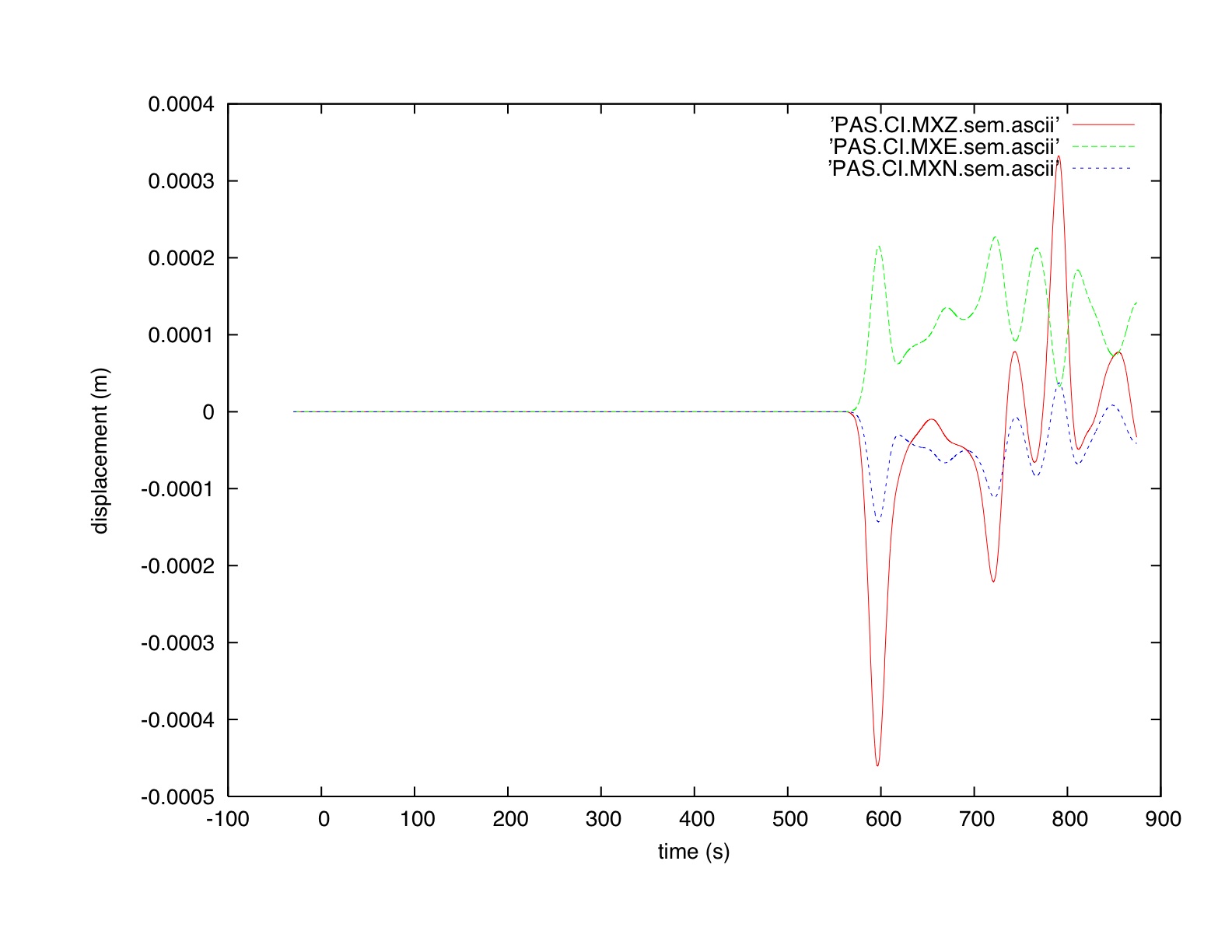
check the output file output_solver.txt in the output directory OUTPUT_FILES/ to see if the forward simulation was successfully finishing. the seismograms for station PAS should look like this, using gnuplot:

gnuplot> plot "PAS.CI.MXZ.sem.ascii" w l,"PAS.CI.MXE.sem.ascii" w l,"PAS.CI.MXN.sem.ascii" w l

This is a step-by-step tutorial how to create a mesh for a regional simulation and run a forward simulation.

The following instructions assume that you have installed SPECFEM3D_GLOBE and familiarized yourself with how you will run the package based on your computer configuration, as detailed in the SPECFEM3D_GLOBE User manual (Chapter 2 provides installation help). Please make sure you have the package installed on your system.

The example is distributed with the package under the EXAMPLES/ directory. However, you might need to edit these example scripts slightly to launch them on your system.

This is a step-by-step tutorial how to create a mesh for a regional simulation and run a single forward simulation.

We will set up the example folder for simulation runs:

* databases directory: create a directory DATABASES_MPI/ into which you will put the mesh partitions:

[]$ cd SPECFEM3D_GLOBE/EXAMPLES/regional_MiddleEast/
[regional_MiddleEast]$ mkdir -p DATABASES_MPI

Make sure this folder is accessible by the compute nodes on your system. The example will search for this folder in the current example directory. Depending on your system setup, you may also create this as a symbolic link to a local scratch directory /scratch/DATABASES_MPI.

* parameter files: make sure you have the parameter files in a local directory DATA/ for the example:

[regional_MiddleEast]$ ls -1 DATA/
Par_file
CMTSOLUTION
STATIONS

these files should already be provided in the example folder.

* executables: Copy the above example parameter files to the DATA/ directory in the root directory before compiling. Then compile the executables in the root directory:

[]$ cd SPECFEM3D_GLOBE/
[SPECFEM3D_GLOBE]$ make

this assumes that you run the configuration beforehand by ./configure (see the manual for further configuration options). In case the compilation was successful, it will create the main executables xmeshfem3D and xspecfem3D in the bin/ directory

Note: the solver executable xspecfem3D uses static allocations which will depend upon the parameters set in the Par_file. According to those parameters, a source header file OUTPUT_FILES/values_from_mesher.h will be created during the compilation process by the executable xcreate_header_file. The solver only runs for those parameter setups.

create a local directory bin/ to link the executables from the root directory:

[]$ cd SPECFEM3D_GLOBE/EXAMPLES/regional_MiddleEast
[regional_MiddleEast]$ mkdir -p bin    
[regional_MiddleEast]$ cd bin/
[bin]$ ln -s ../../bin/xmeshfem3D
[bin]$ ln -s ../../bin/xspecfem3D

All these steps and the following mesher and solver runs are put in a process.sh bash script file in the example folder. You can simply run the script:

[regional_MiddleEast]$ ./process.sh

to do the setup and following steps for you. The script uses a PBS scheduler to submit the corresponding cluster job. Please modify and adapt the script to your needs.

You will need to create the mesh databases before you can run the solver.

1. the example will run the mesher in parallel on 64 CPUs. A script go_mesher_solver_pbs.bash is provided in this example folder to do this via a PBS job scheduler. You may adapt also one of the cluster scripts provided in the SPECFEM3D_GLOBE/UTILS/Cluster/ directory for this purpose.

Note: This example script will submit one single job script which contains both the meshing run and the forward solver run together. This is especially useful in case your DATABASES_MPI folder is only locally accessible on the cluster nodes (e.g. local scratch disk space) and allows you to run both meshing and forward simulation without the need to store all the created mesh database files in a globally accessible repository.

2. make sure, you have the parameter file Par_file in the local directory DATA/. This example will use the following parameter setup for the regional simulation:

# forward or adjoint simulation
SIMULATION_TYPE                 = 1   # 1 = forward, 2 = adjoint, 3 = both simultaneously
NOISE_TOMOGRAPHY                = 0   # 0 = earthquake simulation,  1/2/3 = three steps in noise simulation
SAVE_FORWARD                    = .false.  

# number of chunks (1,2,3 or 6)
NCHUNKS                         = 1 

# angular width of the first chunk (not used if full sphere with six chunks)
ANGULAR_WIDTH_XI_IN_DEGREES   = 45.d0      # angular size of a chunk
ANGULAR_WIDTH_ETA_IN_DEGREES  = 40.d0
CENTER_LATITUDE_IN_DEGREES    = 29.d0
CENTER_LONGITUDE_IN_DEGREES   = 55.d0
GAMMA_ROTATION_AZIMUTH        = 0.d0

# number of elements at the surface along the two sides of the first chunk
# (must be multiple of 16 and 8 * multiple of NPROC below)
NEX_XI                          = 128 
NEX_ETA                         = 128

# number of MPI processors along the two sides of the first chunk
NPROC_XI                        = 8 
NPROC_ETA                       = 8
...
# 3D model
MODEL                           = s29ea
...
# path to store the local database files on each node
LOCAL_PATH                      = ./DATABASES_MPI
...

The number of spectral elements in this single chunk in both XI and ETA directions is 128. To obtain the shortest period resolved in the seismograms, you would determine:

shortest period ~ (256 / NEX_XI ) x (ANGULAR_WIDTH_XI_IN_DEGREES / 90 ) x 17

thus for this example, they are accurate down to approximately 17 s periods.

Once the mesher completed, check the output file OUTPUT_FILES/output_mesher.txt to see if the databases were generated successfully. The output file contains various mesh information, including the time step size used for your forward simulation:

time-stepping of the solver will be:   0.142911725716261

To run a forward simulation, do the following:

1. set an earthquake source by modifying the file CMTSOLUTION in the directory DATA/. this example will use a CMT solution for a shallow earthquake (12.8 km depth) which took place in Iran in December, 2003.

You can obtain more CMT solutions from the Global Centroid-Moment Tensor project catalog.

2. place your stations by modifying the file STATIONS in the directory DATA/. this example will use a very small subset of seismic stations in international networks IRIS/IDA (II) and IRIS/USGS (IU).

You can obtain more station information from the International Federation of Digital Seismograph Networks (FDSN).

Please see the SPECFEM3D_GLOBE User manual for more detailed informations of how to specify the source and stations.

3. make sure, you have the parameter files in the directory DATA/. Most parameters in the Par_file should be set before running the mesher xmeshfem3D. The following parameters are important for this example forward simulation:

# forward or adjoint simulation
SIMULATION_TYPE                 = 1   # 1 = forward, 2 = adjoint, 3 = both simultaneously
NOISE_TOMOGRAPHY                = 0   # 0 = earthquake simulation,  1/2/3 = three steps in noise simulation
SAVE_FORWARD                    = .false.  

# number of chunks (1,2,3 or 6)
NCHUNKS                         = 1
...
# number of MPI processors along the two sides of the first chunk
NPROC_XI                        = 8
NPROC_ETA                       = 8
...
# 3D model
MODEL                           = s29ea

# parameters describing the Earth model
OCEANS                          = .true.
ELLIPTICITY                     = .true.
TOPOGRAPHY                      = .true.
GRAVITY                         = .true.
ROTATION                        = .true.
ATTENUATION                     = .true.

# absorbing boundary conditions for a regional simulation
ABSORBING_CONDITIONS            = .true.

# record length in minutes
RECORD_LENGTH_IN_MINUTES        = 15.0d0
...
# path to store the local database files on each node
LOCAL_PATH                      = ./DATABASES_MPI
...  
# output format for the seismograms (one can use either or all of the three formats)
OUTPUT_SEISMOS_ASCII_TEXT       = .true.  
...

this example will use a single job script go_mesher_solver_pbs.bash to run mesher and solver together. The solver should take about 15 minutes to finish the simulation.

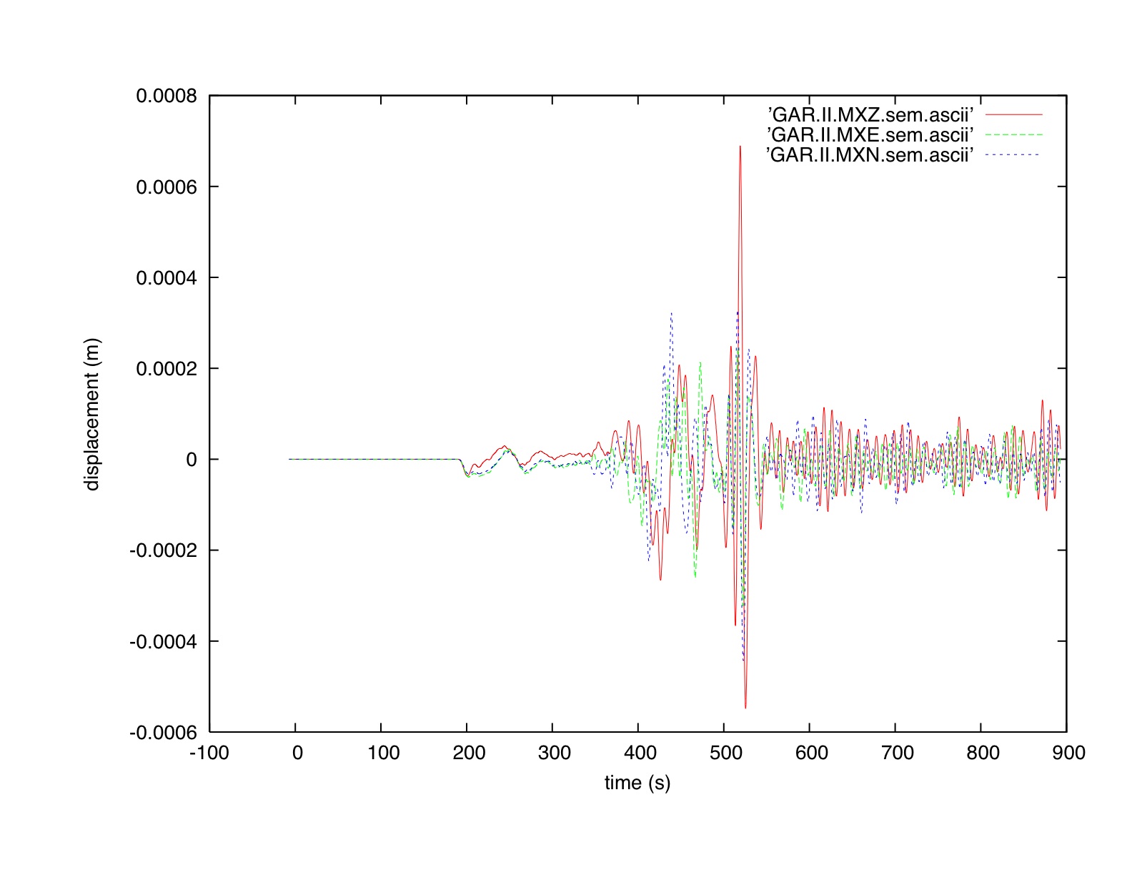
check the output file output_solver.txt in the output directory OUTPUT_FILES/ to see if the forward simulation was successfully finishing. the seismograms for station GAR, located in Garm, Tajikistan, should look like this, using gnuplot:

gnuplot> plot "GAR.II.MXZ.sem.ascii" w l,"GAR.II.MXE.sem.ascii" w l,"GAR.II.MXN.sem.ascii" w l

Benchmark results for SPECFEM3D_GLOBE

We present here a ‘long-period’ (periods longer than 17 s) simulation of a shallow event in isotropic PREM [Dziewonski and Anderson, 1981] without the ocean layer, without attenuation but including the effects of self-gravitation (in the Cowling approximation) (Figures C.1 and C.2).

The normal-mode synthetics are calculated with the code QmXD using mode catalogs with a shortest period of 8 s generated by the code OBANI. No free-air, tilt, or gravitational potential corrections were applied [Dahlen and Tromp, 1998]. We also turned off the effect of the oceans in QmXD.

The normal-mode and SEM displacement seismograms are first calculated for a step source-time function, i.e., setting the parameter half duration in the CMTSOLUTION file to zero for the SEM simulations. Both sets of seismograms are subsequently convolved with a triangular source-time function using the processing script UTILS/seis_process/process_syn.pl.

They are also band-pass filtered and the horizontal components are rotated to the radial and transverse directions (with the script UTILS/seis_process/rotate.pl). The match between the normal-mode and SEM seismograms is quite remarkable for the experiment with attenuation, considering the very different implementations of attenuation in the two computations (e.g., frequency domain versus time domain, constant Q versus absorption bands).

You can download this benchmark example: benchmark_examples.tar.gz (~96 MB).

To unzip the tar ball file, type::

tar -zxvf benchmark_examples.tar.gz

Further tests can be found in the EXAMPLES directory. It contains the normal-mode and SEM seismograms, and the parameters (STATIONS, CMTSOLUTION and Par_file) for the SEM simulations.

Figure C.1: Normal-mode (blue) and SEM (red) vertical displacements in isotropic PREM considering the effects of self-gravitation but not attenuation for 13 stations at increasing distance from the 1999 November 26th Vanuatu event located at 15 km depth. The SEM computation is accurate for periods longer than 17~s. The seismograms have been filtered between 50~s and 500~s. The station names are indicated on the left.

Figure C.2: Same as in Figure C.1 for the transverse displacements

Important remark:

When comparing SEM results to normal mode results, one needs to convert source and receiver coordinates from geographic to geocentric coordinates, because on the equator the geographic and geocentric latitude are identical but not elsewhere. Even for spherically-symmetric simulations one must perform this conversion because the source and receiver locations provided by globalCMT.org and IRIS involve geographic coordinates.

References

F. A. Dahlen and J. Tromp. Theoretical Global Seismology. Princeton University Press, Princeton, New-Jersey, USA, 1998. 

A. M. Dziewonski and D. L. Anderson. Preliminary reference Earth model. Phys. Earth Planet. In., 25:297-356, 1981. 

D. Komatitsch and J. Tromp. Spectral-element simulations of global seismic wave propagation-I. Validation. Geophys. J. Int., 149 (2):390–412, 2002a. doi: 10.1046/j.1365- 246X.2002.01653.x. 

D. Komatitsch and J. Tromp. Spectral-element simulations of global seismic wave propagation-II. 3-D models,oceans,rotation,and self-gravitation. Geophys. J. Int., 150(1):303–318, 2002b. doi: 10.1046/j.1365-246X.2002.01716.x. 

Komatitsch and Tromp [2002a,b] carefully benchmarked the spectral-element simulations of global seismic waves against normal-mode seismograms. Version 4.0 of SPECFEM3D_GLOBE has been benchmarked again following the same procedure.

We present here a ‘short-period’ (periods longer than 9 s) simulation of a deep event in transversely isotropic PREM without the ocean layer and including the effects of self-gravitation and attenuation (Figures C.3, C.4 and C.5).

The normal-mode synthetics are calculated with the code QmXD using mode catalogs with a shortest period of 8 s generated by the code OBANI. No free-air, tilt, or gravitational potential corrections were applied [Dahlen and Tromp, 1998]. We also turned off the effect of the oceans in QmXD.

The normal-mode and SEM displacement seismograms are first calculated for a step source-time function, i.e., setting the parameter half duration in the CMTSOLUTION file to zero for the SEM simulations. Both sets of seismograms are subsequently convolved with a triangular source-time function using the processing script UTILS/seis_process/process_syn.pl.

They are also band-pass filtered and the horizontal components are rotated to the radial and transverse directions (with the script UTILS/seis_process/rotate.pl). The match between the normal-mode and SEM seismograms is quite remarkable for the experiment with attenuation, considering the very different implementations of attenuation in the two computations (e.g., frequency domain versus time domain, constant Q versus absorption bands).

You can download this benchmark example: benchmark_examples.tar.gz (~96 MB).

To unzip the tar ball file, type:

tar -zxvf benchmark_examples.tar.gz

Further tests can be found in the EXAMPLES directory. It contains the normal-mode and SEM seismograms, and the parameters (STATIONS, CMTSOLUTION and Par_file) for the SEM simulations.

Figure C.3: Normal-mode (blue) and SEM (red) vertical displacements in transversely isotropic PREM considering the effects of self-gravitation and attenuation for 12 stations at increasing distance from the 1994 June 9th Bolivia event located at 647 km depth. The SEM computation is accurate for periods longer than 9 s. The seismograms have been filtered between 10 s and 500 s. The station names are indicated on the left.

Figure C.4: Same as in Figure C.3 for the transverse displacements

Figure C.5: Seismograms recorded between 130 degrees and 230 degrees, showing in particular the good agreement for core phases such as PKP. This figure is similar to Figure 24 of Komatitsch and Tromp (2002a). The results have been filtered between 15 s and 500 s.

Important remark:

When comparing SEM results to normal mode results, one needs to convert source and receiver coordinates from geographic to geocentric coordinates, because on the equator the geographic and geocentric latitude are identical but not elsewhere. Even for spherically-symmetric simulations one must perform this conversion because the source and receiver locations provided by globalCMT.org and IRIS involve geographic coordinates.

References

F. A. Dahlen and J. Tromp. Theoretical Global Seismology. Princeton University Press, Princeton, New-Jersey, USA, 1998. 

A. M. Dziewonski and D. L. Anderson. Preliminary reference Earth model. Phys. Earth Planet. In., 25:297-356, 1981. 

D. Komatitsch and J. Tromp. Spectral-element simulations of global seismic wave propagation-I. Validation. Geophys. J. Int., 149 (2):390–412, 2002a. doi: 10.1046/j.1365- 246X.2002.01653.x. 

D. Komatitsch and J. Tromp. Spectral-element simulations of global seismic wave propagation-II. 3-D models,oceans,rotation,and self-gravitation. Geophys. J. Int., 150(1):303–318, 2002b. doi: 10.1046/j.1365-246X.2002.01716.x.